🔵 OpenCV reloaded: Building an Android Diagnostic Strip Scanner

Remember my last post where I fought OpenCV’s HoughCircles over an antibiogram agar plate and completely lost? I promised I’d be back. A year ago. Well, yeah, my fellowship exam happened and my focus was entirely on that for the past few months. Sorry about that. While I originally thought my return would involve heavy machine learning, it turns out that sometimes you don’t need a massive neural network—you just need a better (and easier?) geometric problem to solve.

Instead of trying to find ambiguous circles, I pivoted to a different biomedical challenge: automating the readout of a diagnostic test strip. In our lab we use ViennaLab’s CVD StripAssay, a molecular test strip used to screen patients for inherited genetic risks of cardiovascular diseases, like deep vein thrombosis. It works via reverse hybridization: a patient’s amplified DNA is washed over the strip, binding specifically to the healthy or mutated gene probes fixed inside the 18 lanes and triggering a chemical reaction that turns the line dark.

ViennaLab test strips

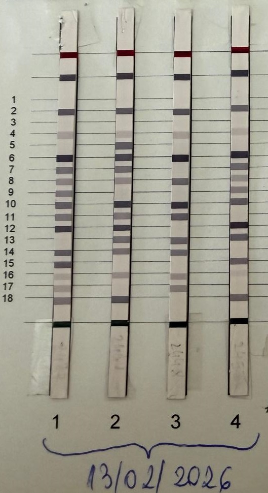
We already have this Windows app called ViennaLab Strip Assay Evaluator but I wanted to see if I could make a more portable app that runs on Android. It’s a nice challenge for me and in the end we’d end up with a phone app that scans the strips and automatically generates the PDF test result. Neat! :)

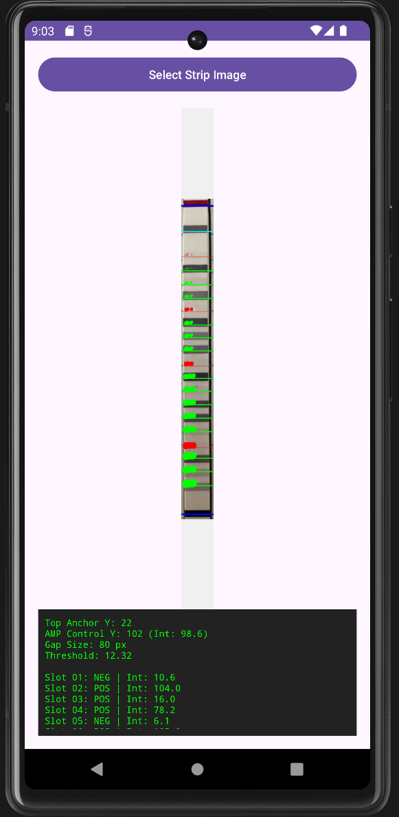The virtual device made in Android Studio running the app

---

📐 The Strategy: Ditching Circles for Linear Profiles

The fundamental flaw with my antibiogram project was relying on edge gradients to fit perfect circles to imperfect, faint biological shapes. Test strips are a different beast entirely. They are inherently linear.

Sooo instead of searching in the dark for shapes, the new “architecture” uses a highly reliable anchor-and-step approach:

1. Find the Structural Anchors: Identify the top and bottom control bands of the strip. These act as our bounding box.
2. Interpolate the Grid: Because the physical strip has 18 evenly spaced test lanes, once we know the exact position of the top and bottom anchors, we can mathematically slice the image into 18 clean, predictable regions of interest (ROIs).
3. Analyze Intensity Profiles: Run a baseline subtraction across each lane. If a specific lane dips below a certain brightness threshold, it means a reaction occurred.

No circle fitting, no floating thresholds, just pure, clean array, ugh, slicing?? 😁

---

🐍 Phase 1: Prototyping in Python

Before jumping into mobile development, I knocked out a quick Python prototype to verify the math. The goal was to take a raw crop of the strip, find the y-coordinates of the structural bands, and iterate through the slots.

import cv2
import numpy as np

TARGET_HEIGHT = 1000
TARGET_WIDTH = 100

# to load the image 
try:
    img_raw = cv2.imread("test.jpg")
    if img_raw is None: raise FileNotFoundError
except:
    img_raw = cv2.imread("testsolo.jpg")

img = cv2.resize(img_raw, (TARGET_WIDTH, TARGET_HEIGHT))
result = img.copy()

gray = cv2.cvtColor(img, cv2.COLOR_BGR2GRAY)
blurred = cv2.GaussianBlur(gray, (5, 5), 0)

raw_signal = 255.0 - np.mean(blurred, axis=1)

def extract_true_paper_baseline(sig, window_size=60):
    baseline = np.zeros_like(sig)
    half_w = window_size // 2
    for i in range(len(sig)):
        start = max(0, i - half_w)
        end = min(len(sig), i + half_w + 1)
        baseline[i] = np.min(sig[start:end])
    return baseline

paper_baseline = extract_true_paper_baseline(raw_signal, window_size=60)
corrected_signal = np.clip(raw_signal - paper_baseline, 0, None)

# 1. Locate the physical geometry markers
y_top_anchor = np.argmax(corrected_signal[:120])
y_bottom_anchor = 880 + np.argmax(corrected_signal[880:])

# 2. Find the AMP Control line first
amp_search_start = y_top_anchor + 40
amp_search_end = y_top_anchor + 160
y_amp_snapped = amp_search_start + np.argmax(corrected_signal[amp_search_start:amp_search_end])

# 3.  Use a 3-pixel local average of the AMP Control for baseline intensity
amp_control_intensity = np.mean(corrected_signal[y_amp_snapped - 1 : y_amp_snapped + 2])

# Calculate the dynamic threshold based strictly on the reactive AMP control line
positivity_threshold = amp_control_intensity * 0.125

true_gap_distance = y_amp_snapped - y_top_anchor

print("--- Calibration Metrics ---")
print(f"Top Anchor Location: Y = {y_top_anchor}")
print(f"Discovered AMP Control Peak: Y = {y_amp_snapped}")
print(f"AMP Control Reference Intensity: {amp_control_intensity:.2f}")
print(f"True Physical Gap Distance: {true_gap_distance} pixels")
print(f"Bottom Anchor Location: Y = {y_bottom_anchor}")
print(f"Dynamic Positivity Threshold (12.5% of AMP): {positivity_threshold:.2f}\n")

y_first_band_geom = y_amp_snapped + true_gap_distance
y_last_band_geom = y_bottom_anchor - true_gap_distance

step_size = (y_last_band_geom - y_first_band_geom) / 17.0
snap_radius = int(step_size * 0.25)

# Render the nchors
cv2.line(result, (0, y_top_anchor), (TARGET_WIDTH, y_top_anchor), (255, 0, 0), 3)
cv2.line(result, (0, y_bottom_anchor), (TARGET_WIDTH, y_bottom_anchor), (255, 0, 0), 3)

# Render the AMP Control
cv2.line(result, (0, y_amp_snapped), (TARGET_WIDTH, y_amp_snapped), (0, 255, 255), 2)
cv2.putText(result, "AMP CONTROL", (10, y_amp_snapped - 6), cv2.FONT_HERSHEY_SIMPLEX, 0.35, (0, 255, 255), 1)

print("--- Array Analysis ---")
for i in range(18):
    y_geometric = int(y_first_band_geom + (i * step_size))
    
    w_start = max(0, y_geometric - snap_radius)
    w_end = min(TARGET_HEIGHT - 1, y_geometric + snap_radius + 1)
    local_window = corrected_signal[w_start:w_end]
    
    local_peak_idx = np.argmax(local_window)
    y_local_peak = w_start + local_peak_idx
    
    peak_intensity = np.mean(corrected_signal[y_local_peak - 1 : y_local_peak + 2])
    
    # Evaluate against the new AMP-driven gate
    if peak_intensity >= positivity_threshold:
        y_final = y_local_peak
        status = "POSITIVE"
        color = (0, 255, 0)
        line_thickness = 2
    else:
        y_final = y_geometric
        status = "NEGATIVE"
        color = (0, 0, 255)
        line_thickness = 1
        
    print(f"Slot {i+1:02d}: {status:8s} | Grid Lane Y: {y_geometric} -> Plotted Y: {y_final} | Intensity: {peak_intensity:.1f}")
    
    cv2.line(result, (0, y_final), (TARGET_WIDTH, y_final), color, line_thickness)
    cv2.putText(result, f"#{i+1:02d} {status[0]}", (10, y_final - 4), 
                cv2.FONT_HERSHEY_SIMPLEX, 0.35, color, 1)

cv2.imwrite("testresult.png", result)

🤖 Phase 2: Shipping it to Android (Kotlin + OpenCV)

I spun up a clean Android Studio project, imported the native OpenCV Android SDK, and vibecoded the processing logic in Kotlin, thanks to Gemini, lol.

// Define our color profiles using OpenCV Scalars (RGBA)
val colorControlBound = Scalar(0.0, 0.0, 255.0, 255.0)  // Blue
val colorPositiveLine = Scalar(0.0, 255.0, 0.0, 255.0)  // Green
val colorNegativeLine = Scalar(255.0, 0.0, 0.0, 255.0)  // Red

// Draw the structural anchor boundaries
Imgproc.line(resizedMat, Point(0.0, yTopAnchor.toDouble()), Point(TARGET_WIDTH.toDouble(), yTopAnchor.toDouble()), colorControlBound, 3)
Imgproc.line(resizedMat, Point(0.0, yBottomAnchor.toDouble()), Point(TARGET_WIDTH.toDouble(), yBottomAnchor.toDouble()), colorControlBound, 3)

// Iterate through the 18 slots and flag their state
for (i in 0 until NUM_SLOTS) {
    val isPositive = analyzeLaneIntensity(resizedMat, i)
    val lineColor = if (isPositive) colorPositiveLine else colorNegativeLine
    
    // Render visual feedback directly onto the bitmap
    Imgproc.rectangle(resizedMat, pointStart, pointEnd, lineColor, 2)
}

🏆 The Takeaway

My first OpenCV venture failed because I tried to force a delicate, highly variable shape algorithm (HoughCircles) to handle ambiguous biological data.

The ThromboStrip app succeeded because I took a step back and reframed the problem. By designing an application around the structural constraints of the test medium itself, traditional computer vision became incredibly robust, lightning-fast, and light enough to run natively on a budget smartphone.

The project code is clean, the colors look sharp, and I don’t have to look at another broken circle parameter constant for a long, long time. 🤣